Example 5.4

Simulation of a continuous-space Markov chain.

import numpy as np
import matplotlib.pyplot as plt

rng = np.random.default_rng(15)

# Note our system x_n = a x_{n-1} + noise
T = 1000
x = np.zeros(T)

x[0] = 100
a = 0.9

for t in range(1,T):
    x[t] = a * x[t-1] + rng.normal(0,1)

plt.plot(x)
plt.show()

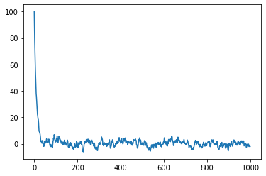
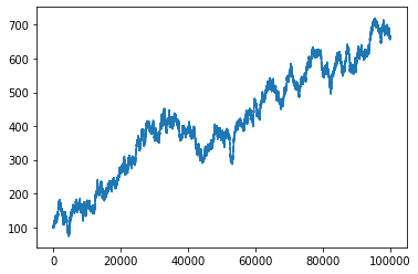
We can see that the chain starts from \(x_0 = 100\) but converges to its stationary measure. For some values \(a\), this may not hold. See the example below with \(a = 1\).

import numpy as np
import matplotlib.pyplot as plt

rng = np.random.default_rng(15)

# Note our system x_n = a x_{n-1} + noise
T = 100000
x = np.zeros(T)

x[0] = 100
a = 1

for t in range(1,T):
    x[t] = a * x[t-1] + rng.normal(0,1)

plt.plot(x)
plt.show()

This chain will not converge anywhere.