Example 3.5

Recall that this example deals with rejection sampling from the posterior distribution.

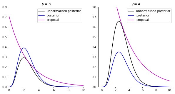
In this example, we have a Gamma prior and a Poisson likelihood as described in the notes. Let us first plot the unnormalised posterior, posterior, and the described proposal in Example 3.5.

import numpy as np
import matplotlib.pyplot as plt

orange_rgb = [0.8, 0.4, 0]


def gamma(x, alpha, beta):
    return (beta**alpha / np.math.factorial(alpha-1)) * x**(alpha-1) * np.exp(-beta * x)

def exponential(x, lam):
    return lam * np.exp(-lam * x)

def Poisson(y, x):
    return np.exp(-x) * x**y / np.math.factorial(y)

def posterior_gamma(x, y, alpha, beta):
    return gamma(x, alpha + y, beta + 1)

def unnormalised_posterior_gamma(x, y, alpha, beta):
    return x**(alpha + y - 1) * np.exp(-beta * x) * np.exp(-x)

def M(x, y, alpha, lam):
    return ((alpha + y - 1)/(2 - lam))**(alpha + y - 1) * np.exp(-(alpha + y - 1)) / (lam)

alpha = 2
beta = 1
y1 = 3
y2 = 4

ylim_max = 0.8
xx = np.linspace(0, 10, 1000)

fig, ax = plt.subplots(1, 2, figsize=(10, 5))
# ax[0].plot(xx, gamma(xx, alpha, beta), 'k-', label='prior')
# ax[0].plot(xx, Poisson(y1, xx), color=[0.8, 0, 0], label='likelihood')
ax[0].plot(xx, unnormalised_posterior_gamma(xx, y1, alpha, beta), color='k', label='unnormalised posterior')
ax[0].plot(xx, posterior_gamma(xx, y1, alpha, beta), color=[0, 0, 0.8], label='posterior')
ax[0].plot(xx, M(xx, y1, alpha, 2/(alpha + y1)) * exponential(xx, 2/(alpha + y1)), 'm-', label='proposal')
ax[0].set_title('$y = 3$')
ax[0].set_ylim([0, ylim_max])
ax[0].set_xlim([0, 10])
ax[0].spines['top'].set_visible(False)
ax[0].spines['right'].set_visible(False)
ax[0].legend()
# ax[1].plot(xx, gamma(xx, alpha, beta), 'k-', label='prior')
# ax[1].plot(xx, Poisson(y2, xx), color=[0.8, 0, 0], label='likelihood')
ax[1].plot(xx, unnormalised_posterior_gamma(xx, y2, alpha, beta), color='k', label='unnormalised posterior')
ax[1].plot(xx, posterior_gamma(xx, y2, alpha, beta), color=[0, 0, 0.8], label='posterior')
ax[1].plot(xx, M(xx, y2, alpha, 2/(alpha + y1)) * exponential(xx, 2/(alpha + y2)), 'm-', label='proposal')
ax[1].set_title('$y = 4$')
ax[1].set_ylim([0, ylim_max])
ax[0].set_xlim([0, 10])
ax[1].spines['top'].set_visible(False)
ax[1].spines['right'].set_visible(False)
ax[1].legend()
plt.show()

<ipython-input-1-7eb21dd97153>:8: DeprecationWarning: `np.math` is a deprecated alias for the standard library `math` module (Deprecated Numpy 1.25). Replace usages of `np.math` with `math`
  return (beta**alpha / np.math.factorial(alpha-1)) * x**(alpha-1) * np.exp(-beta * x)

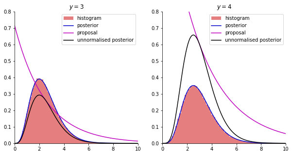
Next, we implement the rejection sampler as described in Example 3.5.

# rejection sampling

def rejection_sampling(N, y, alpha, beta, lam):
    x_accepted = np.array([])
    while len(x_accepted) < N:
        x = np.random.exponential(1/lam)
        u = np.random.uniform(0, 1)
        if u < unnormalised_posterior_gamma(x, y, alpha, beta) / (M(x, y, alpha, lam) * exponential(x, lam)):
            x_accepted = np.append(x_accepted, x)

    return x_accepted

N = 200000
lam_star = 2/(alpha + y1)
alpha = 2
samples_1 = rejection_sampling(N, y1, alpha, beta, lam_star)
lam_star_2 = 2/(alpha + y2)
samples_2 = rejection_sampling(N, y2, alpha, beta, lam_star_2)

fig, ax = plt.subplots(1, 2, figsize=(10, 5))
ax[0].hist(samples_1, bins=100, density=True, color=[0.8, 0, 0], alpha = 0.5, label='histogram')
ax[0].plot(xx, posterior_gamma(xx, y1, alpha, beta), color=[0, 0, 0.8], label='posterior')
ax[0].plot(xx, M(xx, y1, alpha, 2/(alpha + y1)) * exponential(xx, 2/(alpha + y1)), 'm-', label='proposal')
ax[0].plot(xx, unnormalised_posterior_gamma(xx, y1, alpha, beta), color='k', label='unnormalised posterior')
ax[0].set_title('$y = 3$')
ax[0].set_ylim([0, ylim_max])
ax[0].set_xlim([0, 10])
ax[0].spines['top'].set_visible(False)
ax[0].spines['right'].set_visible(False)
ax[0].legend()
ax[1].hist(samples_2, bins=100, density=True, color=[0.8, 0, 0], alpha = 0.5, label='histogram')
ax[1].plot(xx, posterior_gamma(xx, y2, alpha, beta), color=[0, 0, 0.8], label='posterior')
ax[1].plot(xx, M(xx, y2, alpha, 2/(alpha + y2)) * exponential(xx, 2/(alpha + y2)), 'm-', label='proposal')
ax[1].plot(xx, unnormalised_posterior_gamma(xx, y2, alpha, beta), color='k', label='unnormalised posterior')
ax[1].set_title('$y = 4$')
ax[1].set_ylim([0, ylim_max])
ax[1].set_xlim([0, 10])
ax[1].spines['top'].set_visible(False)
ax[1].spines['right'].set_visible(False)
ax[1].legend()
plt.show()

<ipython-input-1-7eb21dd97153>:8: DeprecationWarning: `np.math` is a deprecated alias for the standard library `math` module (Deprecated Numpy 1.25). Replace usages of `np.math` with `math`
  return (beta**alpha / np.math.factorial(alpha-1)) * x**(alpha-1) * np.exp(-beta * x)