Example 2.1#
In what follows, we will implement inversion methods for sampling discrete and continuous distributions.
Discrete distributions#
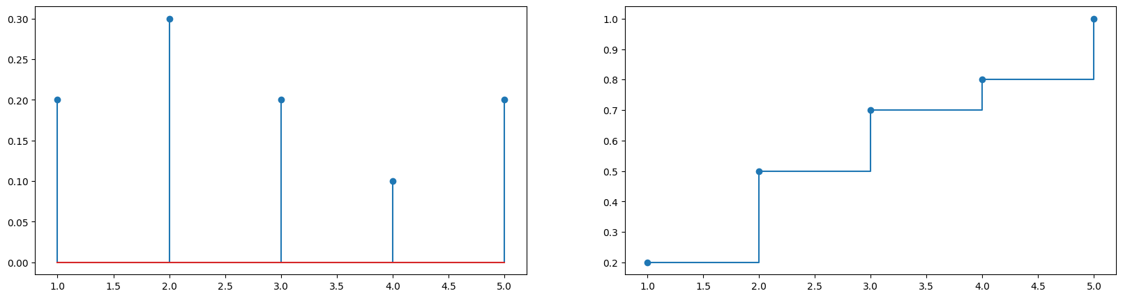
Example 2.1. We think of our discrete distribution very practically as a vector defined on a set of states. Let us define a probability mass function on the set \(\mathsf{S} = \{1, 2, 3, 4, 5\}\) as follows:
Let us plot the PMF and CDF of this distribution.
import numpy as np
import matplotlib.pyplot as plt
w = np.array([0.2, 0.3, 0.2, 0.1, 0.2])
s = np.array([1, 2, 3, 4, 5])
def discrete_cdf(w):
return np.cumsum(w)
cw = discrete_cdf(w)
def plot_discrete_cdf(w, cw):
fig, ax = plt.subplots(1, 2, figsize=(20, 5))
ax[0].stem(s, w)
ax[1].plot(s, cw, 'o-', drawstyle='steps-post')
plt.show()
plot_discrete_cdf(w, cw)
Next, we can implement the sampling method using the inverse. Let us implement the method first, then look into some animations.
import numpy as np
import matplotlib.pyplot as plt
rng = np.random.default_rng(4)
w = np.array([0.2, 0.3, 0.2, 0.1, 0.2])
s = np.array([1, 2, 3, 4, 5])
def discrete_cdf(w):
return np.cumsum(w)
def sample(u, s, w): # discrete sampler for a uniform random variable u, states s and weights w
cdf = discrete_cdf(w)
sample_ind = np.argmax(cdf > u)
return s[sample_ind]
fig, ax = plt.subplots(1, 2, figsize=(10, 5))
n = 2000
x = []
cw = discrete_cdf(w)
un = []
for n in range(n):
u = rng.uniform(0, 1)
un.append(u)
sample_x = sample(u, s, w)
x.append(sample_x)
# the rest is for animation
# plot the pmf using the stem function and change the color of the markers and the line
markerline, stemlines, baseline = ax[0].stem(s, w, markerfmt='o', linefmt='r-')
ax[0].cla()
ax[0].hist(un, bins=10, density=True, color='k', alpha=1)
ax[0].set_title("Histogram of Uniform Random Variables")
ax[1].cla()
ax[1].stem(s, w, markerfmt='o', linefmt='r-')
ax[1].set_xlabel("s")
# plot a histogram centered on states s
ax[1].hist(x, bins=range(7), density=True, color='k', alpha=1, align='mid', width=0.1)
ax[1].set_xlim([0, 6])
ax[1].set_title("Histogram of Discrete Random Variables and PMF")
Text(0.5, 1.0, 'Histogram of Discrete Random Variables and PMF')
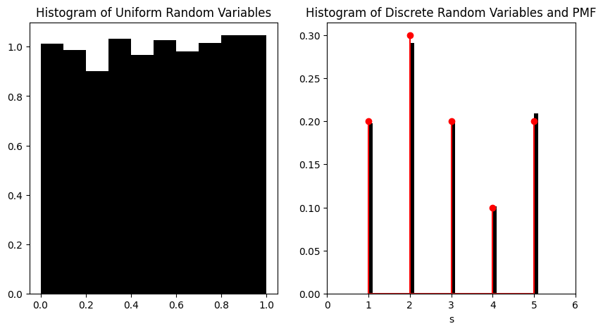
As we can see, with \(n = 2000\), the method samples from the correct distribution. Let us see below this process animated (the code is hidden as it has a lot of diversions from normal code for the sake of animation – but feel free to expand if you are curious!).
Animated discrete sampling#
It is important to visualise these processes to gain intuition. We will first below animate the discrete case, then the continuous case.
Show code cell source
%matplotlib inline
import numpy as np
import matplotlib.pyplot as plt
from matplotlib.animation import FuncAnimation
from IPython.display import HTML, display
rng = np.random.default_rng(7)
w = np.array([0.2, 0.3, 0.2, 0.1, 0.2])
s = np.array([1, 2, 3, 4, 5])
def discrete_cdf(w):
return np.cumsum(w)
def sample(u, s, w): # discrete sampler for a uniform random variable u, states s and weights w
cdf = discrete_cdf(w)
sample_ind = np.argmax(cdf > u)
return s[sample_ind]
fig, ax = plt.subplots(2, 2, figsize=(10, 8))
n = 400
x = []
cw = discrete_cdf(w)
un = []
def update(i):
global un, x
u = rng.uniform(0, 1)
un.append(u)
sample_x = sample(u, s, w)
x.append(sample_x)
# the rest is for animation
if i % 1 == 0:
ax[0, 0].cla()
# plot the pmf using the stem function and change the color of the markers and the line
markerline, stemlines, baseline = ax[0, 0].stem(s, w, markerfmt='o', linefmt='r-')
ax[0, 0].set_title("PMF")
ax[0, 0].set_xlabel("s")
# plot u in the y axis of ax[0, 1]
ax[0, 1].cla()
ax[0, 1].plot(s, cw, 'ro-', drawstyle='steps-post')
ax[0, 1].set_title("Cumulative Distribution Function")
ax[0, 1].set_xlabel("s")
ax[0, 1].set_xlim([0, 6])
ax[0, 1].set_ylim([0, 1])
ax[0, 1].plot(0, u, c='k', marker='o', linestyle='none', markersize=10)
ax[0, 1].plot(sample_x, u, c='k', marker='o', linestyle='none', markersize=10)
ax[0, 1].plot([0, sample_x], [u, u], c=[0.8, 0, 0], linestyle='--')
ax[0, 1].plot(sample_x, 0, c='k', marker='o', linestyle='none', markersize=10)
ax[1, 0].cla()
ax[1, 0].hist(un, bins=10, density=True, color='k', alpha=1)
ax[1, 0].set_title("Histogram of Uniform Random Variables")
ax[1, 1].cla()
ax[1, 1].stem(s, w, markerfmt='o', linefmt='r-')
ax[1, 1].set_xlabel("s")
# plot a histogram centered on states s
ax[1, 1].hist(x, bins=range(7), density=True, color='k', alpha=1, align='mid', width=0.1)
ax[1, 1].set_xlim([0, 6])
ax[1, 1].set_title("Histogram of Discrete Random Variables and PMF")
ani = FuncAnimation(fig, update, frames=n, repeat=False)
HTML(ani.to_jshtml())
Animation size has reached 21019140 bytes, exceeding the limit of 20971520.0. If you're sure you want a larger animation embedded, set the animation.embed_limit rc parameter to a larger value (in MB). This and further frames will be dropped.