Metropolis-Hastings algorithm

Metropolis-Hastings algorithm#

As we have seen in the slides, for a generic target $π (x) \propto γ (x)$ and a proposal $q (x^{'} | x)$ , the Metropolis-Hastings algorithm is defined as follows. Given the state of chain $x_{n - 1}$ , one iteration of this method goes as follows:

Sample $x^{'}$ from $q (x^{'} | x_{n - 1})$
Compute the acceptance probability $α (x_{n - 1}, x^{'}) = min (1, \frac{π (x^{'}) q (x_{n - 1} | x^{'})}{π (x_{n - 1}) q (x^{'} | x_{n - 1})})$
Sample $u \sim U (0, 1)$
If $u < α (x_{n - 1}, x^{'})$ , set $x_{n} = x^{'}$ , otherwise set $x_{n} = x_{n - 1}$
Repeat

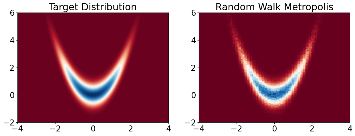
Let us try this on the Banana density example. Recall that this density is defined on $R^{2}$ and is given by

\begin{array}{r} π (x) \propto \exp (- \frac{x_{1}^{2}}{10} - \frac{x_{2}^{2}}{10} - 2 (x_{2} - x_{1}^{2})^{2}) . \end{array}

In this case, we have the unnormalised density

\begin{array}{r} γ (x) = \exp (- \frac{x_{1}^{2}}{10} - \frac{x_{2}^{2}}{10} - 2 (x_{2} - x_{1}^{2})^{2}) . \end{array}

We will now choose our proposal as the random walk proposal

\begin{array}{r} q (x^{'} | x) = N (x^{'}; x, σ_{q}^{2} I), \end{array}

where $σ_{q}^{2}$ is a parameter that we can tune. We will also choose the initial state of the chain to be $x_{0} = (0, 0)$ .

Note that, since $q (x^{'} | x) = q (x | x^{'})$ , the acceptance probability simplifies to

\begin{array}{r} α (x_{n - 1}, x^{'}) = min (1, \frac{π (x^{'})}{π (x_{n - 1})}) . \end{array}

The following code implements the Metropolis-Hastings algorithm for the Banana density.

import numpy as np
import matplotlib.pyplot as plt

rng = np.random.default_rng(24)

# banana function for testing MCMC
def log_gamma(x):
    return -x[0]**2/10 - x[1]**2/10 - 2 * (x[1] - x[0]**2)**2

N = 1000000
samples_RW = np.zeros((2, N))

# initial values
x_1 = 0
x_2 = 0
samples_RW[:, 0] = np.array([x_1, x_2])
# parameters
gamma = 0.005

sigma_rw = 0.5

burnin = 200

for n in range(1, N):
    # random walk
    x_s = samples_RW[:, n-1] + sigma_rw * np.random.randn(2)
    # metropolis
    u = rng.uniform(0, 1)

    if np.log(u) < log_gamma(x_s) - log_gamma(samples_RW[:, n-1]):
        samples_RW[:, n] = x_s
    else:
        samples_RW[:, n] = samples_RW[:, n-1]


# for surf plot banana 2d
x_bb = np.linspace(-4, 4, 100)
y_bb = np.linspace(-2, 6, 100)
X_bb, Y_bb = np.meshgrid(x_bb, y_bb)
Z_bb = np.exp(log_gamma([X_bb, Y_bb]))

plt.figure(figsize=(15, 5))
# make fonts bigger
plt.rcParams.update({'font.size': 20})
plt.subplot(1, 2, 1)
cnt = plt.contourf(X_bb, Y_bb, Z_bb, 100, cmap='RdBu')
plt.title('Target Distribution')

plt.subplot(1, 2, 2)
plt.hist2d(samples_RW[0, burnin:n], samples_RW[1, burnin:n], 100, cmap='RdBu', range=[[-4, 4], [-2, 6]], density=True)
# remove the white edges from plt.hist2d
plt.title('Random Walk Metropolis')
plt.show()

../_images/9293e6dd80774599afbf91151919a0735dcc7ca2b0b03a36be8d6cb23f8c1668.png