Sampling via Inversion#
A simple example of sampling via inversion will be given below.
In the lecture we have derived the sampler for exponential distribution:
\[\begin{align*}
p(x) = \text{Exp}(x;\lambda) = \lambda e^{-\lambda x}.
\end{align*}\]
We calculate the CDF
\[\begin{align*}
F_X(x) =& \int_{0}^x p(x') \mathrm{d} x', \\
=& \lambda \int_0^x e^{-\lambda x'} \mathrm{d} x', \\
=& {\lambda} \left[ -\frac{1}{\lambda} e^{- \lambda x'}\right]_{x' = 0}^x \\
=& 1 - e^{-\lambda x}.
\end{align*}\]
Deriving the inverse:
\[\begin{align*}
u =& 1 - e^{-\lambda x}\\
\implies x =& -\frac{1}{\lambda} \log (1 - u)\\
\implies F_X^{-1}(u) =& -\lambda^{-1} \log (1 - u).
\end{align*}\]
which gives us the sampler:
Generate \(u_i \sim \text{Unif}([0, 1])\)
\(x_i = -\lambda^{-1} \log (1 - u_i)\).
Let us look at the code for this sampler.
import numpy as np
import matplotlib.pyplot as plt
rng = np.random.default_rng(10)
def exponential_pdf(x, lam):
return lam * np.exp(-lam * x)
def exponential_cdf(x, lam):
return 1 - np.exp(-lam * x)
# an illustration of inverse transform sampling for the exponential distribution
# with parameter lambda = 4
lam = 4
N = 50000
x = np.array([])
un = []
for n in range(N):
u = rng.uniform(0, 1)
un.append(u)
x = np.append(x, -np.log(1 - u) / lam)
fig = plt.figure(figsize=(10, 5))
axs = fig.subplots(1, 2)
# plot u on the y axis
xx = np.linspace(0, 2, 100)
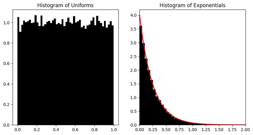
axs[0].hist(un, bins=50, density=True, color='k') # histogram of uniforms
axs[0].set_title("Histogram of Uniforms")
axs[1].hist(x, bins=50, density=True, color='k') # histogram of exponentials
axs[1].plot(xx, exponential_pdf(xx, lam), color=[0.8, 0, 0], linewidth=2) # plot the pdf
axs[1].set_xlim(0, 2)
axs[1].set_title("Histogram of Exponentials")
plt.show()