The Kalman filter

The model below is taken from the paper, Section 5.3 with simplifications.

We consider the model in the paper, and the first part of this code concerns with data generation.

import numpy as np
import matplotlib.pyplot as plt

rng = np.random.default_rng(1234)

# define the linear system for object tracking
# x = [x, y, vx, vy]
T = 1000
x = np.zeros((4, T))
x[:, 0] = np.zeros(4)

k = 0.04

A = np.block([
    [np.eye(2), k * np.eye(2)],
    [np.zeros((2, 2)), 0.99 * np.eye(2)]
])

Q = np.block([
    [k**3 / 3 * np.eye(2), k**2 / 2 * np.eye(2)],
    [k**2 / 2 * np.eye(2), k * np.eye(2)]
])

H = np.array([[1.0, 0.0, 0.0, 0.0], [0.0, 1.0, 0.0, 0.0]])

R = 0.1 * np.array([[1, 0.0], [0.0, 1]])

y = np.zeros((2, T))

for t in range(1, T):
    x[:, t] = A @ x[:, t-1] + rng.multivariate_normal(np.zeros(4), Q)
    y[:, t] = H @ x[:, t] + rng.multivariate_normal(np.zeros(2), R)

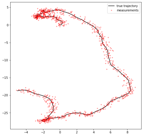
fig = plt.figure(figsize=(8, 8))

plt.plot(x[0, :], x[1, :], 'k-')
plt.plot(y[0, :], y[1, :], 'r.', alpha=0.3)
plt.legend(['true trajectory', 'measurements'])

<matplotlib.legend.Legend at 0x12c87db20>

Next, as explained in the slides, we write our Kalman filtering functions.

def kalman_predict(mu, V, A, Q):
    mu_pred = A @ mu
    V_pred = A @ V @ A.T + Q
    return mu_pred, V_pred

def kalman_update(mu_pred, V_pred, H, R, y):
    S = H @ V_pred @ H.T + R
    K = V_pred @ H.T @ np.linalg.inv(S)
    mu = mu_pred + K @ (y - H @ mu_pred)
    V = V_pred - K @ H @ V_pred
    return mu, V

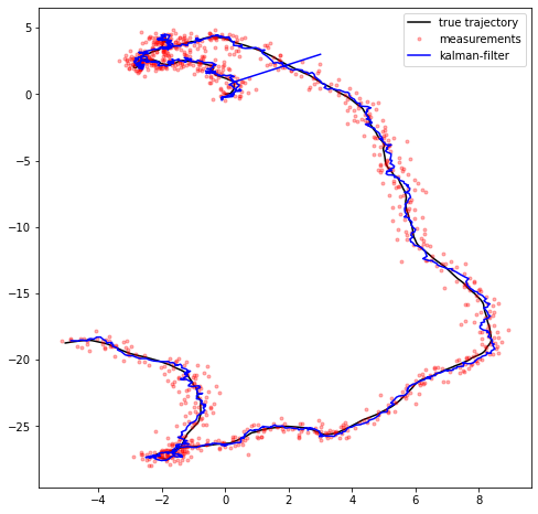
Next, we will run our filter - and compare the filter estimates to the ground truth signal.

mu = np.zeros((4, T))
V = np.zeros((4, 4, T))

mu[:, 0] = np.ones(4) * 3
V[:, :, 0] = 10 * np.eye(4)

mu_pred = np.zeros((4, T))
V_pred = np.zeros((4, 4, T))

for t in range(1, T):
    mu_pred[:, t], V_pred[:, :, t] = kalman_predict(mu[:, t-1], V[:, :, t-1], A, Q)

    mu[:, t], V[:, :, t] = kalman_update(mu_pred[:, t], V_pred[:, :, t], H, R, y[:, t])

plt.figure(figsize=(8, 8))
plt.plot(x[0, :], x[1, :], 'k-')
plt.plot(y[0, :], y[1, :], 'r.', alpha=0.3)
plt.plot(mu[0, :], mu[1, :], 'b-')
plt.legend(['true trajectory', 'measurements', 'kalman-filter'])
plt.show()